For this week’s assignment, I chose this pattern to recreate,
and here is my recreation of this art.
For this week’s assignment, I chose this pattern to recreate,
and here is my recreation of this art.
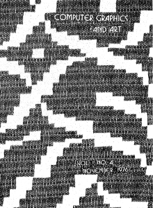
For my Computer Graphics art recreation project (see on the top below), I decided to attempt to faithfully recreate the following image (on the bottom below) from the 1978 issue of Computer Graphics and Art:
Choose.
That is the only instruction, along with three circles of different color, on the “menu” page, the default starting page of my drawing machine. My intention was to create a program which gives the users a sense of discovery and surprise.
Here’s the code from class
I am a psychology major and thus encounter Gaussian distributions quite a lot. That is why I decided to recreate Terry Jones’s piece entitled – you guessed it – “Gaussian distribution”.
Terry Jones: “Gaussian Distribution”
Miha Klasinc: “Terry Jones’s Gaussian Distribution”
Processing facilitated my job quite a lot since it provided me with a built-in Gaussian distribution function. The function outputs a number following standardized normal distribution. This means that there is a roughly 68% probability that the outputted number is within one standard deviation (i.e. 1 unit) away from the mean 0, a 95% probability that the number is within two standard deviations away from the mean etc. If the function is called a number of times (e.g. 10000 times), a relatively uniform distribution of values clustered around the mean emerges. I created a for loop that calls the Gaussian distribution function 20000 times. Upon each iteration, a small circle is created. The first circle’s X coordinate is set to 1 and then increases by 1 with each iteration. If the X value exceeds the limits of the canvas the X coordinate is set back to 0. The circles’ Y coordinates are determined by the addition of outputted random numbers to half of the canvas’ size. This results in circles being distributed around the line that splits the canvas into two equal halves.
Here’s the code:
int xCoordinate = 1;
int canvasHeight = 400;
float middleLine = canvasHeight/2;

void setup() {
  size(800, 400);
  background(255);
}

void draw(){
  stroke(0);
  fill(0);
}


void GaussianDistr(){
  for(int i = 0; i < 20000; i++){
    float y = randomGaussian() * 50;
    ellipse(xCoordinate,middleLine+y,2,2);
    xCoordinate++;
    if(xCoordinate >= width){
      xCoordinate = 0;
    }
    println(xCoordinate);
    redraw();
  }
}

void mousePressed() {
  GaussianDistr();
  redraw();
  saveFrame("GaussianDistribution.png");
}
I find this particular image interesting among all the old computer graphics available:
Code:
size(700, 500);
int x = 0;
int y = 0;
for(int i = 0; i < 5; i++){
   for(int j = 0; j < 7; j++){
     rect(x, y, 100, 100);
     float limit = random(2, 10);
     for(int k = 0; k < limit; k++){
       float offset = k+5*k+5;
       float xTemp = x+offset;
       float yTemp = y+offset;
       float size = (limit-k)*10;
        rect(xTemp, yTemp, size, size);
        xTemp+=5;
        yTemp+=5;
     }
     x+=100;
   }
   x = 0;
   y+=100;
}
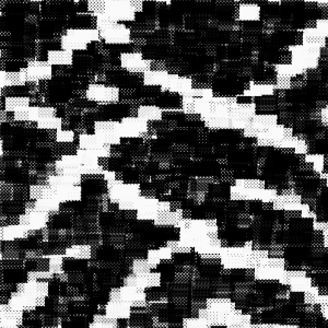
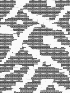
I chose to try and recreate the Manfred Mohr Computer Graphic in two different ways; first by using for loops to create the black patterning, and the second way by using a pattern as a drawing tool to create the image.
void setup(){
  size(600,800);
  background(250);
  for(int j = 0; j <800; j+=5){
  for (int i = 0; i <600; i+=5) {
    line(i,0+j,5+i,5+j);
    line(i,5+j,5+i,0+j);
  }
  }
  for(int j = 0; j<800; j+=5){
  for(int i = 0; i<600; i+=5){
    if(j % 50 == 0){
  for(int w = 0; w<15; w+=5){
      line(i,w+j,5+i,(w+5)+j);
    line(i,(w+5)+j,5+i,w+j);
  }
    }
  }
  }
   for(int j = 0; j<800; j+=15){
  for(int i = 0; i<600; i+=15){
    if(j % 15 == 0){
    strokeWeight(1.5);
      line(i,j,5+i,5+j);
    line(i,5+j,5+i,j);
    }
  }
   }
    for(int j = 0; j<800; j+=10){
  for(int i = 0; i<600; i+=10){
    if(j % 30 == 0){
      strokeWeight(2.5);
      stroke(225);
      line(i,j,5+i,5+j);
    line(i,5+j,5+i,j);

    }
  }
    }

}
void draw(){
float x = mouseX;
float y = mouseY;
if (mousePressed == true){
  stroke(250);
  line(x,y,x+5,y-5);
  line(x,y-5,x+5,y);
  line(x+5,y,x+10,y-5);
  line(x+5,y-5,x+10,y);
  line(x+10,y,x+15,y-5);
  line(x+10,y-5,x+15,y);
  line(x+15,y,x+20,y-5);
  line(x+15,y-5,x+20,y);
  line(x+20,y,x+25,y-5);
  line(x+20,y-5,x+25,y);
  line(x+25,y,x+30,y-5);
  line(x+25,y-5,x+30,y);
  line(x+30,y,x+35,y-5);
  line(x+30,y-5,x+35,y);
  line(x+35,y,x+35,y-5);
  line(x+35,y-5,x+35,y);

  line(x,y,x+5,y+5);
  line(x,y+5,x+5,y);
  line(x+5,y,x+10,y+5);
  line(x+5,y+5,x+10,y);
  line(x+10,y,x+15,y+5);
  line(x+10,y+5,x+15,y);
  line(x+15,y,x+20,y+5);
  line(x+15,y+5,x+20,y);
  line(x+20,y,x+25,y+5);
  line(x+20,y+5,x+25,y);
  line(x+25,y,x+30,y+5);
  line(x+25,y+5,x+30,y);
  line(x+30,y,x+35,y+5);
  line(x+30,y+5,x+35,y);

  line(x,y+5,x+5,y+10);
  line(x,y+10,x+5,y+5);
  line(x+5,y+5,x+10,y+10);
  line(x+5,y+10,x+10,y+5);
  line(x+10,y+5,x+15,y+10);
  line(x+10,y+10,x+15,y+5);
  line(x+15,y+5,x+20,y+10);
  line(x+15,y+10,x+20,y+5);
  line(x+20,y+5,x+25,y+10);
  line(x+20,y+10,x+25,y+5);
  line(x+25,y+5,x+30,y+10);
  line(x+25,y+10,x+30,y+5);
  line(x+30,y+5,x+35,y+10);
  line(x+30,y+10,x+35,y+5);

  line(x,y+10,x+5,y+15);
  line(x,y+15,x+5,y+10);
  line(x+5,y+10,x+10,y+15);
  line(x+5,y+15,x+10,y+10);
  line(x+10,y+10,x+15,y+15);
  line(x+10,y+15,x+15,y+10);
  line(x+15,y+10,x+20,y+15);
  line(x+15,y+15,x+20,y+10);
  line(x+20,y+10,x+25,y+15);
  line(x+20,y+15,x+25,y+10);
  line(x+25,y+10,x+30,y+15);
  line(x+25,y+15,x+30,y+10);
  line(x+30,y+10,x+35,y+15);
  line(x+30,y+15,x+35,y+10);
  }
}
And this is just a small graphic I made while playing around with Processing
Browsing through different graphics generated by computer programs, I found one piece from Edward Zajec very interesting. It is the first piece of a series of graphics called The Cube: Theme and Variation Series. In this graphic, the combination of geometric shapes builds a three-dimensional architecture on a two-dimensional plane. Zajec’s work can be divided into four layers or four parts. Every part is not closely connected, so the graphic shows different layers of the foundation of a huge architecture.
Here’s my recreation of Zajec’s piece. It’s not one-hundred-percent proportional to Zajec’s piece.